2 Setting up an R environment
2.1 The Essentials
2.1.1 For Windows
2. Input the following: which allows us to use more complex packages and tools.
3. Input the following to make sure that 2. has worked:
Sys.which("make")4. Verify that the output to 3. is:
#>                               make
#> "C:\\rtools43\\usr\\bin\\make.exe"
5.Install RStudio(Free Version)
You are ready to install packages
2.2 A Deeper Dive
Setting up an R environment is quite a grandiose way of saying we’ll install R and another program that will make working with R easier - RStudio. It’s easy, quick and free. We just need to follow a few steps in sequence, note; the sequence is important here so make sure you install things in the correct order.
Firstly, we’ll install R on our machine. For this demonstration I will be using RStudio as my Integrated Development Environment (IDE) (and I recommend you do too). 2 out of the 3 machines I run are Windows (the third is Linux) so I’ll demonstrate the installation in Windows and explain how installing on Mac or Linux differs.
RStudio offers a supportive environment in which to learn R analysis, with a comprehensible file structure, the ability to see and export plots and charts as well as access to markdown and notebook formats (, which is the document format used to create this document).
2.3 Installing R
Installing R is very simple. The latest version of R is always available at https://cloud.r-project.org/. Choose the correct version for your hardware (either Linux, Mac or Windows)
Figure 2.1: Download the correct R version for your operating system
Choose the base version for now as this is probably the first time that you’re installing R and finally you can download the latest version of R, in this case version 4.2.0. When you’re downloading the version number may be higher. That’s fine. You should download the latest version available.
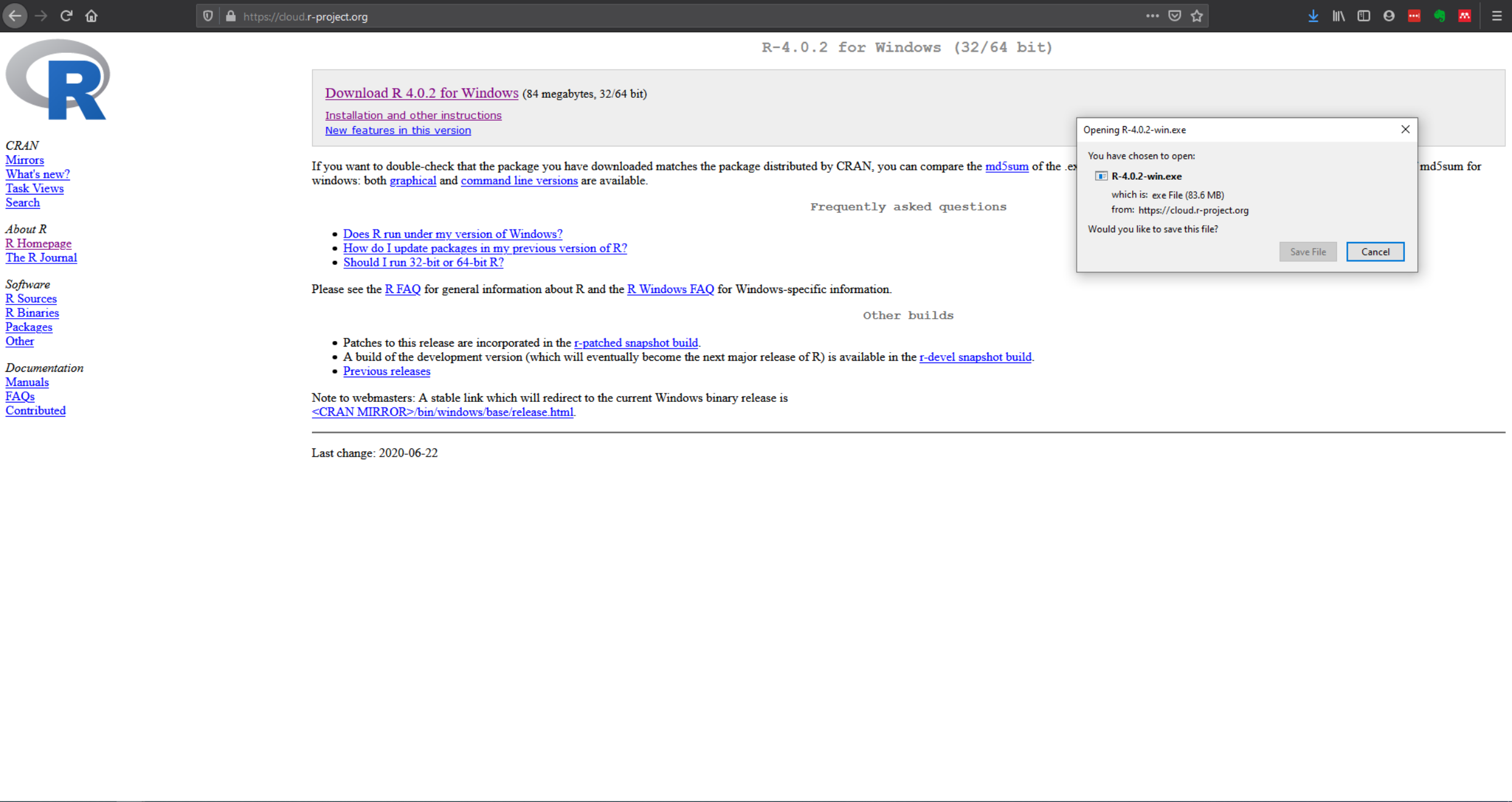
Figure 2.2: Download the latest version of R. The version you download may be higher than the one pictured
Save the file and install the program, choosing your native language, agreeing to the license and choosing a place to install. Don’t change the default installation place unless you have a good reason to (and know what you’re doing).
Each version of R will install separately so you can have multiple different versions on your computer at once. This can occasionally be useful if a package (an add-on for R that provides more functionality) is no longer maintained and only works with an older version. You can keep the older version for the old package but use a newer version for all your other analyses.
2.4 Using R
Now you can open R. You’ll see one window, displaying generic information about your R version and a blinking cursor.
Figure 2.3: The interface for R is rudimentary but totally functional
This is the base R language and you could use this window alone for your complete analysis. However, it can get quite confusing typing in long scripts into the command line and it can be very error prone. We’ll use an Integrated Development Environment (IDE), which helps organise files, see outputs and more easily and generally streamline the process of using a programming language. The IDE we’ll be using is RStudio. Lets install RStudio now.
2.4.1 Installing the development environment
In addition to RStudio, many of the R libraries and algorithms that we will use come from diverse sources. They are not a core part of the R programming language but add-ons. We will need to make R capable of reading these libraries and algorithms in. For this we will need to install additional development tools and make sure that R has access to them
2.4.1.1 For Windows
Install the Rtools add-on for from CRAN repository. If you have R 4.2 click here to download the tool you need
Once it’s installed we’ll need to run the following command in your console
writeLines('PATH="${RTOOLS40_HOME}\\usr\\bin;${PATH}"', con = "~/.Renviron")Close and reopen R (do NOT save the work-space)
We’ll need to verify that R can locate Rtools successfully so run the following line in the
Console(you can just copy and paste it):
Sys.which("make")- If everything is working correctly you should see the following output returned in the
Console:
#>                               make
#> "C:\\rtools43\\usr\\bin\\make.exe"
The above lines are a good demonstration of how the rest of this tutorial will work. The first ‘code block’ shows the entered commands. You can copy and paste these to your console and hit Enter. The second code block shows the results of the commands and you can compare your results to mine.
2.4.1.2 For Mac
You’ll need to make sure that you
Have XCode installed; it can be gotten from here: https://developer.apple.com/xcode/resources/.
Add a FORTRAN compiler see here to get the latest version and any other instructions required.
2.4.1.3 For Linux
You’ll need to install the development version of R in addition to the core version.
If you already have R installed then you can just run
apt-get install r-base-dev (This version is for Ubuntu, change the packet manager command(’apt-get install in this case) depending on your Linux flavour)
2.5 Installing an Integrated Development Environment - RStudio
As mentioned, it is possible to work with just the R installation console to run a full analysis. However, that can be a frustrating and difficult experience. An Integrated Development Environment (IDE) adds many tools and layers of organization to make the analysis simpler and easier to understand. It offers a supportive environment in which to learn R analysis with a comprehensible file structure, the ability to see and export plots and charts as well as access to markdown and notebook formats (which this tutorial was written in). Markdown allows us to combine code snippets with normal text to write reports to write complex reports including all the code and figures created. It’s a great way to present and explain your data whilst showing your working.
You can install RStudio here. It’s free and quite small.
Figure 2.4: There are many different RStudio versions but the Free flavour will do everything we need. The paid versions are used primarily by corporate clients.
2.6 Preparing our workspace
For this demonstration I will be using RStudio as my Integrated Development Environment (IDE) (and I recommend you do too). It offers a supportive environment in which to learn R analysis with a comprehensible file structure, the ability to see and export plots and charts as well as access to markdown and notebook formats. The auto-complete code functions also speed up and streamline your coding.
Here’s what my Rstudio looks like:
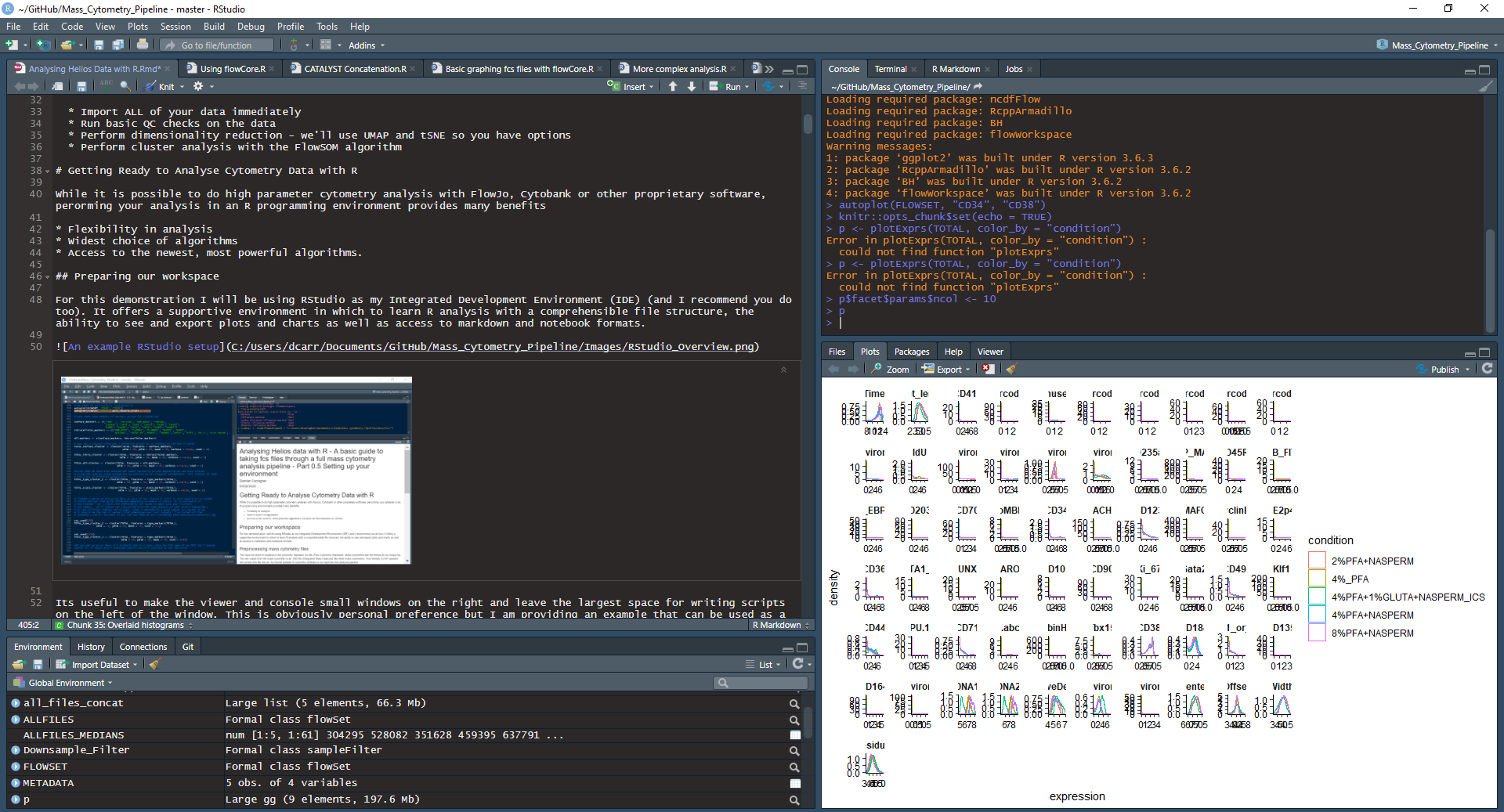
Figure 2.5: WHat your RStudio might look like when you’re finished
Yours will look different. There are 2 important ways to change the appearance to suit you. I’ve provided my layout but if you don’t like it choose an appearance or layout that suits you. It’s best to be comfortable with our environment. If you’re not sure what you like yet, use my settings and then change it as your preferences change.
AppearanceAccessed via theTools>Global Optionsmenu Choose the general colour and theme that offers the best clarityPanesAccessed from theViewmenu Allows you to put each of the 4 sub-windows where you want. TheView>Panes>Panes Layoutmenu allows even finer control on where and how you put the each of the windows and what tabs are included in each.
Figure 2.6: The Panes menu offers the opportunity to place each of the 4 workspace windows where you want
Also, remember that you can resize each of the windows with the mouse as required.
Figure 2.7: The Panes menu offers the opportunity to place each of the 4 workspace windows where you want
Now you’ve gotten the appearance as you wish, we can explore the functions of each and how they might help your analysis. The environment consists of 4 windows that can be used to view several different aspects of your analysis simultaneously. Let’s start at the top right window and go around clockwise:
2.6.1 Top Right (CONSOLE, Terminal and Jobs)
Figure 2.8: The top right pain consists of the Console, Terminal and Jobs tabs, echo = FALSE
2.6.1.1 Console
The console is exactly the same as in the R program we used earlier - when you first open RStudio you should see the version of R that you are running noted in the console window. You can use this window to type out R commands and they will be interpreted as soon as you hit enter
Figure 2.9: The console works exactly like the R interface we tested earlier after installing R for the first time.
Its useful to make the viewer and console small windows on the right and leave the largest space for writing scripts on the left of the window. This is obviously personal preference but I am providing an example that can be used as a starting point for anyone. You can change the windows in Rstudio using the ‘View’ menu and then choosing options from the Panes option - for instance. Console on Right
2.6.1.2 Terminal
TheTerminal provides access to the System Shell like bash or PowerShell. If you haven’t heard of these, don’t worry, we won’t be using them in this guide but it is there if you want to use it. Common uses of the shell are
- remote log-in
- file management - If you need to copy files from elsewhere you can do it without leaving RStudio, which is often quicker
- version control - I sometimes use it to initiate Git (a version control program)
(#fig:Console Video2)The console works exactly like the R interface we tested earlier after installing R for the first time.
2.6.1.3 Jobs
The Jobs tab is where we can monitor Background Tasks or Jobs we’ve assigned R to do. It is often used for handling interactions of R with
- Databases (e.g. SQL)
- Spark (a separate programming language specifically designed to handle big data)
- Run scripts - we can assign R scripts to run in the background.
The most likely use for new users is to run scripts in the background. You can install packages or run large scripts in the background using the jobs window. As we’ll see in this course, if we run taxing algorithms in the foreground, we can ’t continue to use R/RStudio until the analysis task is complete. If we turn the work into a background job we can let the analysis complete while we continue to work on our code or layouts.
Figure 2.10: The console works exactly like the R interface we tested earlier after installing R for the first time.
2.6.2 Bottom Right (Files, Plots, Packages, Help, Viewer)
2.6.2.1 Files
The Files tab works similar to File explorer. It reveals the structure of you project folder and the types of files inside. You can drag and drop files into this pain and they will be added to the current folder. You can also create or delete folders without the need to leave Rstudio.
Figure 2.11: The Files pane allows standard file managmemt processes adn checjing your file organisation
2.6.2.2 Plots
The plots window is where all of the plots you make in the console will be shown. If you make multiple plots you can scroll through them with the small arrow icons.
Figure 2.12: The Plots viewer in action
2.6.2.3 Packages
The Packages tab shows all of the packages that have previously been installed and provides a helpful way to update them if needed. It is also searchable to check if a particular package is installed. We’ll specifically look at Packages in the next chapter.
2.6.2.4 Help
Each package generally comes with basic instructions and example code to help you get up and running. These are called vignettes. You can access these files in RStudio by entering either help(PackageName) or ?PackageName so if we want to pull up the help for flowCore we can enter ?flowCore and see the introduction and menu for all of flowCore’s commands and functions. If you want help in a less specific way you can use ?? which activates the help.search() function. This searches all of the help files and installed-package materials for mentions of the keyword.
Figure 2.13: The Plots viewer in action
2.6.3 Bottom Left Environment etc.
In the bottom left corner we have the Environment along with tabs for History, Connections (and possibly Build and Tutorial)
2.6.3.1 Environment
The Environment tab keeps track of objects (any data frames or tables we may have improted or created) and variables (lists of values we’ve assigned to an arbitrary name) that we are using in our analysis. You can also use the Import Dataset option to easily import common data sets (like excel,csv or SAS). We won’t be using this as part of this tutorial but it can be a useful option. What we will be using the Environment tab for is to keep track of files and objects we create to make sure our analysis is procedding as expected. The figure below shows how each file or variable we assign populates the environment tab and provides info about its type
Figure 2.15: As we create a variable and import a table we can see the Environment tab populate with their name and some basic info.
2.6.3.2 History
History is a straightforward list of all of the commands you have entered into the console throughout your project. If you’ve forgotten what commands (or order) you’ve used you can track that here.
2.6.3.3 Connections
Connections is somewhat beyond the remit of this tutorial. Briefly, it shows the links you have made using R to databases and other complex data sources, either local or remote.
2.6.3.4 Build
Build may not always be present. It depends on the types of packages you have installed and what you are using RStudio to do. In this case the Build tab is here to allow “building” a large document (like this tutorial). It can be safely ignored for most of our analyses. If you start using Rmarkdown documents for your reporting you might start taking advantage of it.
2.6.4 Conclusion
So that’s a whirlwind tour of RStudio, which we’ll be using for the rest of the tutorial. Hopefully we’ve introduced all of the different features, tabs and windows that RStudio offers and briefly explained what each of them does. You’ll begin to understand more of these features as we work our way through the analysis.